Can contrastive identification survive biological data?
Exploring whether shared environmental forcing can be surmounted by contrastive identification methods like DYSCO, and whether they can recover latent states from biological data.
Background
A few things motivating this post, which is the first entry in my “Fables” exercise:
This observation by Marc-Andre Schulz that linear models seem to beat NNs when noise is high, which aligns with my biases but seems to contradict advice shared at the deep learning for science workshop I attended last week. Is biology to complicated for AI or not?
Muratore et al (2606.13260) and associated LinkedIn post: introduce DYSCO to recover the latent state of a complex system, applying it to fMRI data. The key idea is that it only trains on shared views of a given observations, whcih would include snapshots of a system under a chaning environment. What caught my eye is this worked even given uncertainty; the plots in her post reminded me of time series.
I wanted to know if Muratore’s approach could stand up to the degree of uncertainty we commonly observe in biological data, and if it could be used to recover latent states from those systems for which we either are darn sure about the shape of the underlying dynamics or are uncertain whether there is a deterministic state at all.
Problem Statement
DYSCO and it’s ancestor DYNCL are specialized models used to recover latent states from observations. They’re a form of symbolic regression, which is a type of machine learning that aims to find mathematical expressions that best fit the data. The key idea behind DYSCO is to identify contrastive features in the data that can help distinguish between different latent states.
In ecology and the life sciences, we have non-linear processes arising in dynamic environments that give rise to noisy data (that we don’t observe perfectly to begin with). We also have strong assumptions, often in the form of mechanistic models, that underlie all kinds of fields (e.g., population dynamics, epidemiology, etc.). My question is whether DYSCO can be applied to these types of data and still recover meaningful latent states.
Setup
I had four system “case studies” in mind:
Bacterial growth (logistic/Gompertz). This is a simple, low-dimensional system that is well-characterized. The observation challenge here is that we have two views: optical density (OD) readings and plate counts. This case tests recovery at the simple end — what’s the minimum data requirement?
Fisheries Stock-recruit relationship. This is a nonlinear, noisy, regime-dependent system. The observation challenge is that we have two survey types. This case tests recovery when the signal is weak and biologically contested.
Lotka-Volterra predator-prey. This is an oscillatory system. The observation challenge is that we have two species observation channels. This case tests recovery of coupled dynamics (+ the paper validates on oscillatory regimes).
SIR epidemic model. Threshold behavior system. The observation challenge is that we have case counts and seroprevalence as views. This case tests recovery near a dynamical threshold.
…And then, in keeping with my Fable exercise, I threw this at Claude Fable. Prompt is here12, resultant code is here.
Fabled findings
I’ll paste some key things that Claude3 reported back, then add my comments.
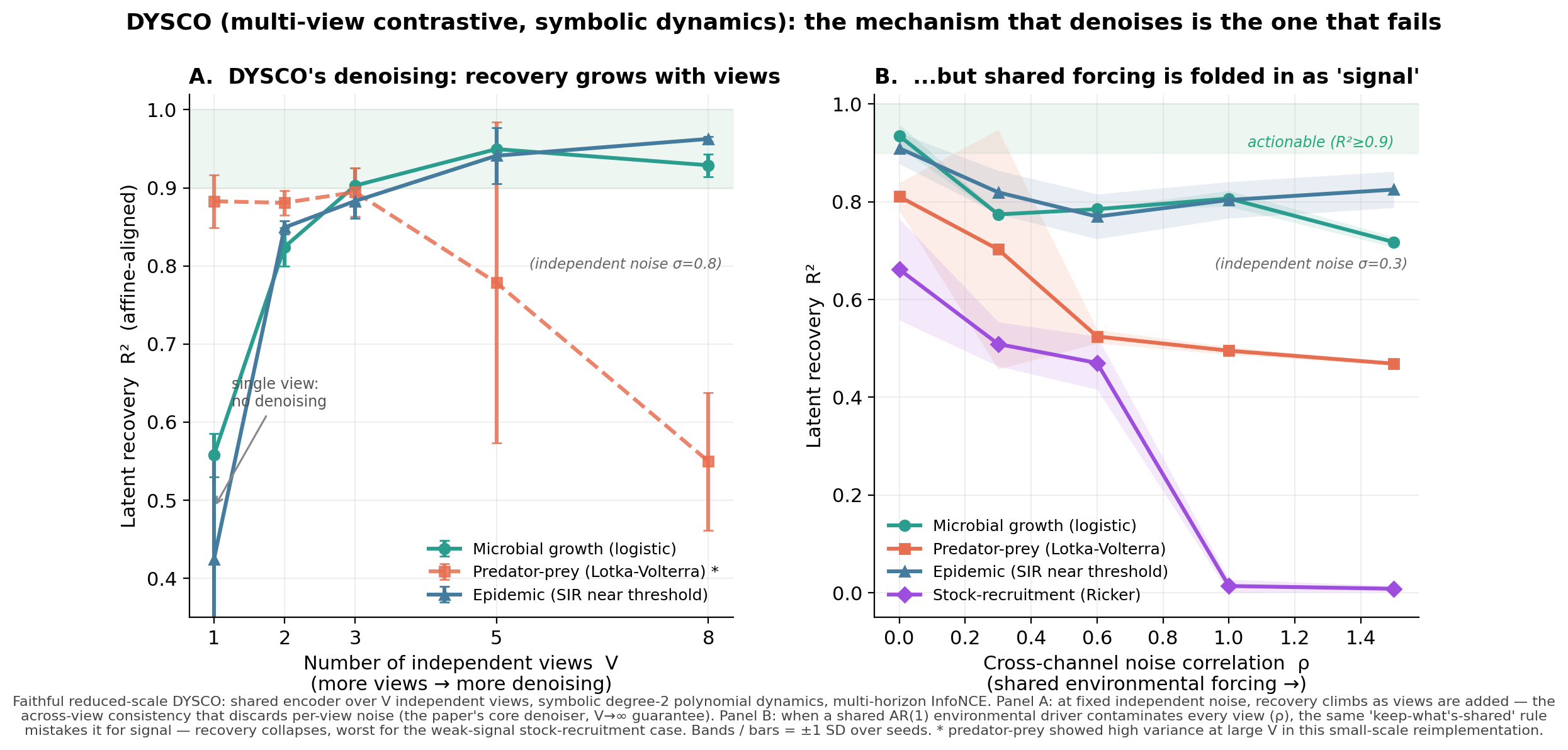
Claude writes:
DYSCO’s denoising strength and its blind spot are the same mechanism.
Panel A confirms the paper’s claim on its own terms. Under heavy independent measurement noise (σ=0.8), a single view fails badly (R²≈0.42–0.56), but recovery climbs steeply as you add independent views (→0.93–0.96 by V=5–8). That’s the V→∞ guarantee working as advertised.
Panel B is the honest catch. DYSCO denoises by keeping what’s shared across views. A shared environmental driver is, by definition, shared across views — so DYSCO mistakes it for signal and folds it into the latent. Recovery degrades exactly as in v1, and stock-recruitment (weak signal) collapses to R²≈0 once the shared driver dominates (ρ≥1). More views don’t help here; they make it worse, because every extra view carries the same confound.””
The better uncertainty handling is real, but it buys robustness only against the noise the theorem assumes (independent across views). Against shared environmental forcing — the thing ecologists actually have — the sophistication doesn’t rescue you, and can hurt. That’s a cleaner “when does it earn its place” argument than v1 alone.
My findings
This tells me that the intuition we’ve long had about life science data is clargely correct: that most shared environmental forcing can’t be surmounted by such multi-channel views and should probably be handled explicitly.
HOWEVER…I had to poke it to make a heatmap (decomposition of results along the cross-channel correlation and measurement noise axes) to actually show there is a frontier here:
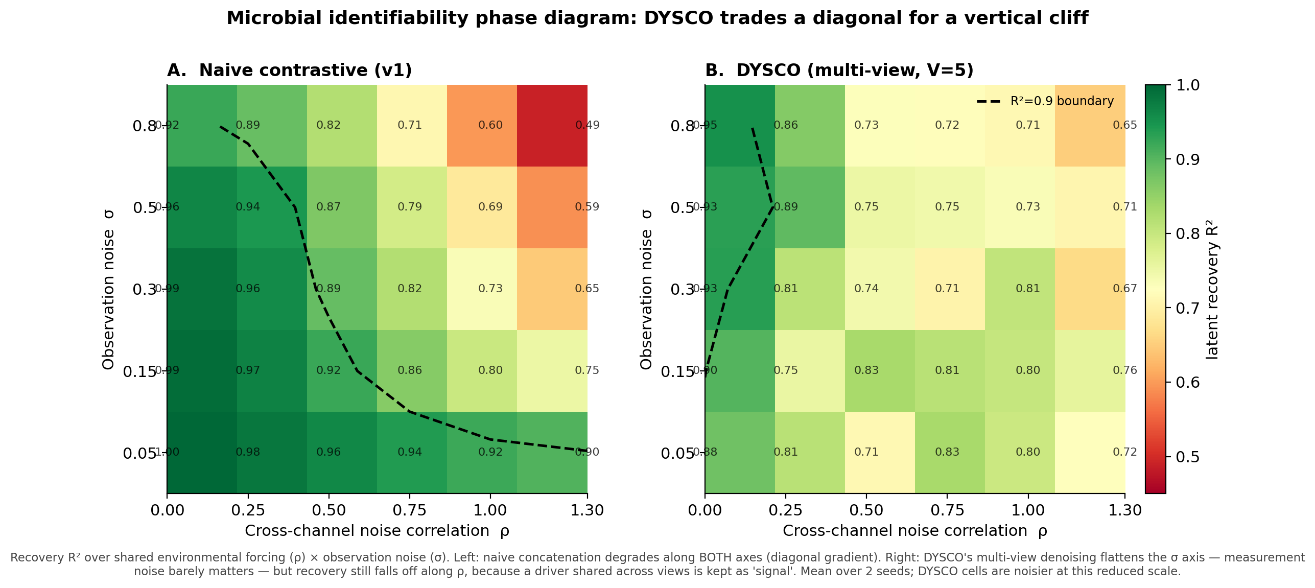
…The paper’s guarantee is that the latent state can be recovered with enough views, and the heatmap shows that this is only true when the shared forcing is low. Once the shared forcing is high, the recovery collapses, and more views don’t help. So the clean tradeoff I would’ve inferred from the DYNCL results (lhs) seem to break down for DYSCO (rhs)., and suggest the frontier is a) more complex and yet b) more heavily driven by the shared forcing, which aligns with my intuition about biological data. There is a encouraging amount of green on that plot.
We often think about these as one singular dimension, or that the cross-channel correlation (here, \(\rho\)) is something that must be explicitly modeled (as we handle in or autoregressive models for geospatial inferences). I’m seeing now that we should consider these as separate and we can get great recovery if only one of them is high (good experimental design insight).
In retrospect, it’d be nice to come up with a few more examples like the stock-recruit, in which we a not so sure that there is a deterministic latent state; the dropoff in latent recovery with uncertainty is striking (especially given that ~0.6 is considered a super great (low) value for \(\rho\) in production).
Cover image is Figure 1 from Muratore et al (2606.13260). Source
Footnotes
By happy accident I forgot to attach the PDF the first time and Claude did the whole exercise using a minimal DYNCL approach, and concluded that method could sufficiently recover the latent state with a clear relationship between channel correlations and observation noise. It found a rapid dropoff in recoverability for the stock-recruit relationship specifically, and produced the lhs of the figure above.↩︎
The prompt I gave to Claude Fable: “There is a recent paper showcasing the DYSCO model by Muratore et al. I want to stress test it. The goal is to produce a concise illustration of my desired case studies (below) that I can share on a blog post. You can keep the tech and assumptions as simple as possible. Don’t check in until you have a plot to share, but check in if you hit 30% usage. Contrastive learning methods for dynamical system identification — exemplified by DYSCO and its predecessor DYNCL — offer theoretical guarantees for recovering latent states and governing dynamics from multiple noisy observation channels, up to an affine transformation. These guarantees are compelling but rest on asymptotic assumptions and have been validated primarily in physics-inspired systems under relatively controlled simulation conditions. Whether they hold up against the kind of data that biologists and ecologists actually collect remains an open question — and answering it honestly is what this paper does. We systematically stress-test contrastive dynamical system identification across a suite of biological systems spanning distinct dynamical regimes and data realities: microbial growth dynamics (simple, monotone, tractable to scale), predator-prey oscillations (cyclic, partially observed), epidemic spread near a threshold (metastable, aggregated counts), and stock-recruitment relationships (weak nonlinear signal, chronically data-limited). Each system is chosen not just as an application domain but as a representative of a distinct identifiability challenge. Using simulation infrastructure drawn from ecological modeling practice — operating model / estimation model design with explicit noise structures — we characterize the boundaries of recovery as a function of time series length, noise level, sampling frequency, and crucially, the degree of correlation in noise across observation channels. The last of these directly targets a core assumption of the framework that is routinely violated in biological systems through shared environmental forcing. For microbial systems, where data collection is tractable at scale, we develop a phase diagram of identifiability — mapping where recovery succeeds, degrades gracefully, or fails — and connect this to thresholds for autonomous experimental decision-making. We ask: when is the residual affine indeterminacy small enough to be scientifically actionable, and what additional observations most efficiently reduce it? The goal is not to propose a new algorithm but to provide the life sciences community with an honest, domain-grounded answer to a practical question: when does this class of AI-driven system identification actually earn its place in your workflow, and when are you better off with a well-specified mechanistic model. The key is choosing systems that span a meaningful axis — not just”look, it works on different things,” but systems that vary along dimensions that matter for the methodology: Lotka-Volterra predator-prey, Bacterial growth (logistic/Gompertz), SIR epidemic model, Stock-recruit relationship.↩︎
My Claude Max account re-routed this to Opus 4.8 but I’m keeping the name for the sake of the series.↩︎