Why do we use ln(19)?
Have you ever noticed that sneaky \(log(19)\) in your logistic equation for maturity or selectivity? What is up with that?
Let’s take the example of a basic selectivity-at-age function, which uses the parameters \(a_{50}\) and \(a_{95}\). These represent the ages where a fish has a probability 50% or 95% chance of being captured. Read that again carefully. I took these parameters for granted, but the meaning of them is intertwined with the use of \(ln(19)\), and if they change, so does the logged value.
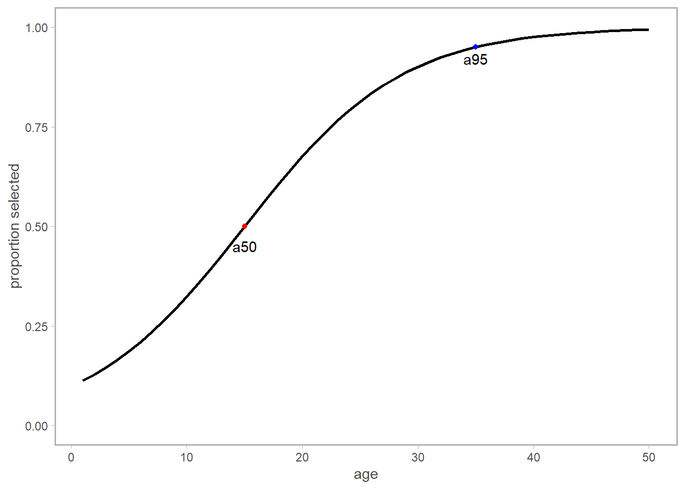
Here’s a selectivity plot with some made up numbers. The selectivity function I’m using is:
\[ S_a = \langle 1+exp(-log(19)*\frac{a-a_{50}}{a_{95}-a_{50}}) \rangle ^{-1} \]
Note how nicely these values extend between zero and one (on the y axis)? That’s because we’re really interested in working with the odds of being captured. Based on our parameter definitions, we need to ensure that the logistic function equals 0.95 when \(a = a_{95}\) (and similarly equals 0.5 at \(a_{50}\)). To achieve this, we recognize the exponent of the log odds equals the odds ratio. You can think of the odds ratio as the probability of your event (getting captured) happening over the probability of it not happening. We can leverage this to force the logistic equation to scale the way we want.
Since we’ve already defined \(a_{95}\) as the age at which we have a 95% probability of getting captured, the log-odds can be defined as \(log(\frac{0.95}{0.05})\). This could be rewritten as \(log(\frac{19/20}{1/20})\) and simplifies to \(log(19)\). This ensures that when \(a = a_{95}\), the equation up top indeed returns 0.95, which is the logistic function evaluated at an odds ratio of 95%.
Given this syntax you’ll see how we would never really need to correct for \(a_{50}\), since the odds ratio of two events with 50% probability is actually zero (plug in 0.5 to see for yourself).
Two notes:
Sometimes to ease model fitting, we will simplify the above equation by substituting \(\delta\) in place of the denominator (\(a_{95} - a_{50}\)), or estimate \(\delta\) as \(\frac{ln(19)}{a_{95} - a_{50}}\). (Specifically, if you have the \(a_{50}\) and \(\delta\) values from, say, a Stock Synthesis model, you can solve for \(a_{95}\) via \(a_{95} = \frac{-ln(19)}{\delta}+a_{50}\)).
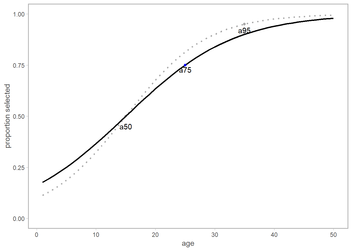
If you’d want to use the something like \(a_{75}\), you’d need to update the log odds via \(log(\frac{0.75}{0.25})\) or ~ \(log(3)\). Note that this ensures that you are getting a 75% selectivity at the corresponding age, but provides a distinct curve from before.